Structure stays exact; constants train
The compiler takes the model as text, an S-expression in a 51-operation first-order language, and emits a frozen PyTorch module that reproduces the program to floating-point precision. Named constants become trainable parameters; everything else is fixed.
From equation to module
A scientist who knows the form of a law but not its constants writes it directly
as a program. The damped pendulum
θ″ = −(g/L) sin θ − b θ′
becomes the two-line Scheme expression on the right. A single call,
compile_scheme(source, inputs={...}), turns it into a frozen
nn.Module in under 150 µs. The constants g_L and
b are exposed as nn.Parameter entries, so ordinary gradient descent
fits them against data while the compiled structure, including the transcendental
sin, computes exactly everywhere on its safe domain.
Because the input is a string, modules are systematically generable: changing
"(sin x)" to "(exp (sin x))" yields a new correct module instantly,
and libraries of compiled equations can be chained or recombined without writing new PyTorch
code. The language covers scalar arithmetic (24 ops), vector operations (9), matrix operations
(11), and control flow (7), enough for ODE right-hand sides and PDE discretizations.
; damped pendulum acceleration
;   theta'' = -(g/L) sin(theta) - b theta'
; g_L and b compile to trainable parameters
(- (* (- 0 g_L) (sin theta))
   (* b theta_dot))
The whole model. Two trainable scalars, one transcendental, no weights to initialize, nothing to approximate.
Parse
Recursive-descent parsing of S-expressions into an
AST. Bracket syntax [1 2 3] desugars to (vec 1 2 3).
A-Normal Form
Compound subexpressions are let-bound to fresh temporaries, giving a one-to-one map from bindings to graph nodes.
Tail-call optimization
Tail-recursive time-stepping and fixed-point loops are rewritten as iteration, so scientific loops execute efficiently.
Graph → DirectModule
Each binding becomes a node in a dataflow DAG,
compiled to a PyTorch nn.Module that evaluates in topological order and
broadcasts over batches.
Hard constraints against four baseline families
Six experiments: 15 Feynman physics laws, two ODE systems (Lotka-Volterra and a damped pendulum), a 1D heat equation, compositional generalization, and 3D vector mechanics, each compared against hand-coded PyTorch, PINN, Neural ODE, and pure MLP baselines.
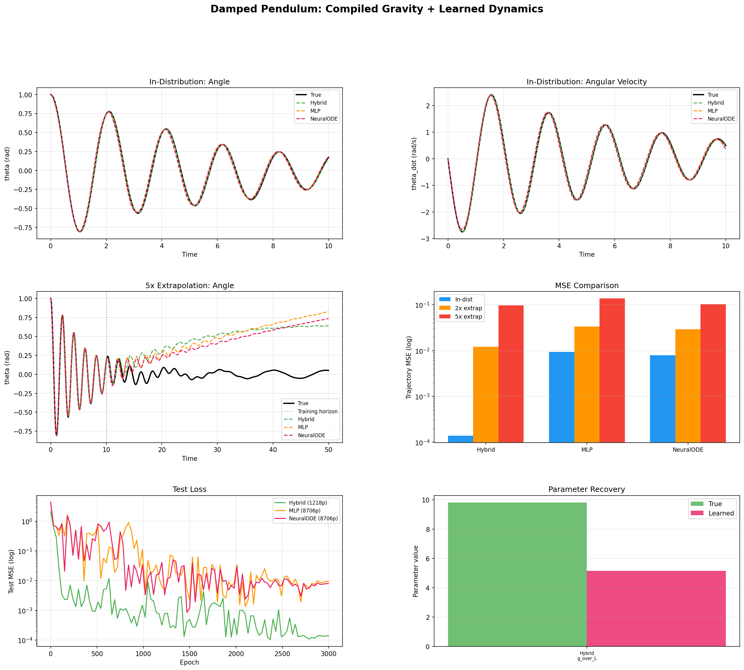
Damped pendulum: 2 parameters against 8,706
The pendulum's transcendental sin term is exactly what MLPs
approximate poorly outside their training range. The full-structure compiled model, just the
two constants g_L and b, recovers g/L to 0.08% error and achieves
731× better in-distribution trajectory MSE than the 8,706-parameter MLP, and
3,000× better at 5× extrapolation (5.0×10⁻⁶ vs
1.5×10⁻²). The PINN baseline (8,580 parameters) recovers g/L with
41.1% error: the soft physics penalty is insufficient for the nonlinear dynamics.
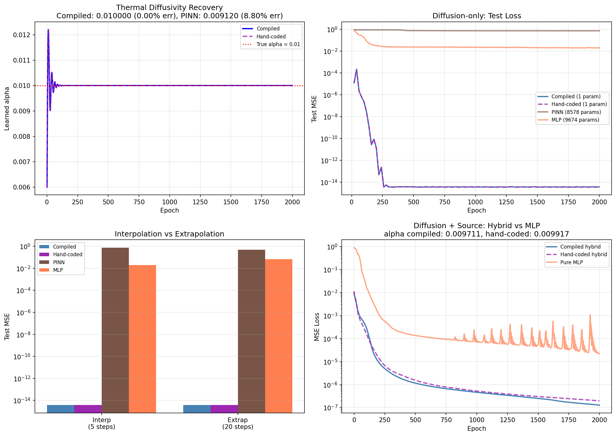
Heat-equation inverse problem: hard vs soft constraints
The heat equation ut = α∇²u is discretized on 10 grid points with the compiler's matrix operations, leaving a single trainable parameter, the thermal diffusivity α. The compiled and hand-coded models recover α with 0.00% error (test MSE near 10−15). The PINN, with 8,578 parameters, shows 92.7% diffusivity error: the soft physics penalty lets the network fit the data without learning the constant. This is the starkest hard-vs-soft constraint gap in the paper.
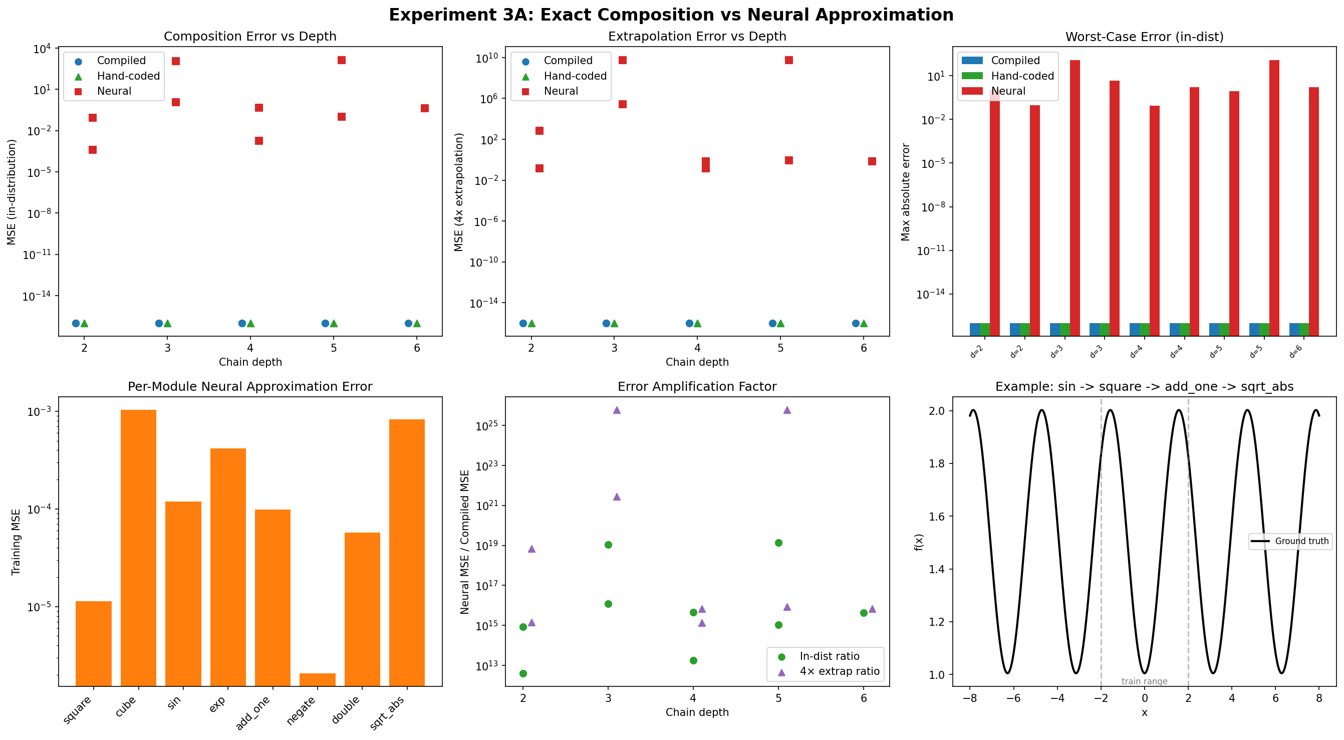
Composition without error accumulation
Chains of depth 2 to 6 built from eight compiled operation modules compose with exactly zero error, in-distribution and at 4× extrapolation. Chains of the corresponding trained MLP approximations accumulate errors up to 5.9 × 10⁹: per-module approximation error is amplified by the Lipschitz constants of downstream modules.
Scope, honestly stated
These are six experiments with hand-coded PyTorch, PINN, Neural ODE, and pure-MLP baselines, not a survey. For any single fixed equation the compiled module is numerically identical to a careful hand-coded implementation; the compiler's contribution is systematic generation and composability, not accuracy over hand-coding. Two of the 15 Feynman equations fail to recover constants (the harmonic oscillator's periodic loss landscape and the Lorentz factor's singularity), optimization failures rather than compilation failures. And compiled hybrid training costs 2.5 to 3.8× more wall-clock time than a pure MLP.
One graph per program
The Neural Compiler established that exact, differentiable structure beats soft constraints. Its own design also marked the boundary the next paper had to cross.
Limitation First-order only
The source language excludes closures, higher-order functions, and general data structures, and supports recursion only in restricted forms (tail calls compile to loops; other recursion runs under a bounded-depth dispatch). Full Scheme programs are out of reach.
Limitation Programs are the compiled artifact
Every new equation is staged into its own graph. The program stops being data the moment it is compiled, so exploring many candidate structures means one compilation per candidate, and nothing at runtime can propose or rewrite programs.
The observation that became Paper 2
The compiler is expressive enough to compile something more useful than any single model: a Scheme interpreter written in Scheme. Compile that interpreter once and every program it runs becomes data, inheriting differentiability with no recompilation and no per-program reimplementation. That is DMCI, Paper 2 of this program; the full arc is traced in the program lineage.
Read it, run it, cite it
The paper, the open-source compiler, and the next chapter of the program.
The paper →
The Neural Compiler: Program-to-Network Translation for Hybrid Scientific Machine Learning. arXiv:2605.22498.
The code →
The compiler, the 51-operation language, all six experiments, and the baselines. github.com/sheneman/neural_compiler
Next: DMCI →
Compile Once, Differentiate Everywhere. The successor paper compiles the interpreter, not the program. arXiv:2606.09930.
Cite this paper
@article{sheneman2026neuralcompiler,
  title         = {The Neural Compiler: Program-to-Network Translation
                   for Hybrid Scientific Machine Learning},
  author        = {Sheneman, Lucas},
  year          = {2026},
  journal       = {arXiv preprint arXiv:2605.22498},
  eprint        = {2605.22498},
  archivePrefix = {arXiv}
}