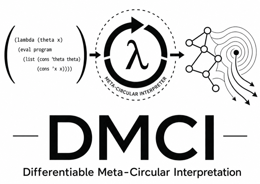
The compiled object is a reusable Scheme evaluator. New programs are supplied as data and automatically inherit differentiability, without recompilation, custom gradients, or reimplementation.
Known structure, unknown constants
Scientists often know the form of a model (Coulomb's law, a decaying exponential, a coupled recurrence) but not its exact constants, and sometimes not even which structural variant is right. DMCI does not compete head-to-head with neural networks; it makes executable scientific models directly optimizable against data, and searchable.
Existing approaches
Fixed scientific code
Exact structure, but its constants are tuned by hand. You cannot gradient-optimize the unknowns; every parameter becomes a manual sweep.
exact · manual tuningNeural networks
Learned structure, but an opaque internal representation of physics you may already know. Data-hungry, and weak at extrapolation.
learned · opaqueDifferentiable frameworks
Exact gradients (PyTorch, JAX, Zygote, Enzyme), but each model must be re-implemented in the framework before it can be differentiated.
exact · per-model effortCompile a differentiable interpreter once. Express scientific models as executable programs. Optimize their continuous parameters directly through interpreted execution, and let a search propose the structures.
- One compiled evaluator serves every runtime-supplied program, no per-model reimplementation
- Exact reverse-mode gradients reach the constants inside any program it runs
- Programs are data, so a search loop can explore structures while gradients fit parameters
Structure frozen, constants learned
A program's structure (its control flow, recursion, composition) stays fixed while its numeric constants become trainable parameters fit by gradient descent. This erases the boundary between fixed scientific programs and gradient-optimized parameters. Where exact structure is known, that structural inductive bias helps: in one inverse heat-equation benchmark from the Neural Compiler paper, encoding the known equation let gradient descent recover the diffusivity accurately where a physics-informed neural-network (PINN) baseline struggled, an illustration of structural prior, not a claim of universal superiority over PINNs.
Where is differentiation located?
Existing systems differentiate an individual model or program; each new model must be re-implemented in the framework first. DMCI is best understood by where it locates differentiation: the differentiated object is a compiled, self-hosting interpreter.
| System | What is differentiated? | New model needs reimplementation? |
|---|---|---|
| PyTorch | Individual model | Yes |
| JAX | Individual program | Yes |
| Zygote | Individual program | Yes |
| Enzyme | Individual program | Yes |
| Differentiable interpreters | Hand-built interpreter | Often (hand-engineered) |
| DMCI | Compiled meta-circular interpreter | No |
DMCI moves differentiation from the model level to the interpreter level, the central conceptual shift of the paper.
Program-and-Parameter Co-Search
A language model (e.g. via OpenEvolve,
an open implementation of AlphaEvolve,
 Google DeepMind's
Gemini-powered coding agent) searches the discrete space of program structures;
DMCI's exact gradients search each program's continuous parameters. Because every
runtime-supplied program inherits differentiability from one frozen interpreter, the two close into
a single joint structure-and-parameter discovery loop, with no per-program reimplementation.
Google DeepMind's
Gemini-powered coding agent) searches the discrete space of program structures;
DMCI's exact gradients search each program's continuous parameters. Because every
runtime-supplied program inherits differentiability from one frozen interpreter, the two close into
a single joint structure-and-parameter discovery loop, with no per-program reimplementation.
What gradients optimize
- Continuous constants
- Tensor parameters
- Numerical coefficients
Optimized by DMCI's exact reverse-mode gradients, taken only with respect to the bound parameter tensors.
What gradients do not optimize
- Program syntax
- Control-flow structure
- Interpreter dispatch
Structure is searched externally, by an LLM, OpenEvolve, or evolutionary search. Keeping the two distinct is essential.
Battery capacity fade: co-search recovers a degradation law Exp L
From a smooth square-root seed (which cannot express a "knee"), the co-search rediscovers a knee-capable structure from the generating family on mechanism-labeled synthetic cells, and improves held-out extrapolation on real Severson lithium-ion cells. Held-out RMSE after a rigorous 300-step DMCI calibration of each candidate (lower is better).
| Synthetic (knee target) | Knee? | RMSE |
|---|---|---|
| Smooth √t seed | no | 0.0301 |
| Hand two-reservoir (true family) | yes | 0.0143 |
| Hand sigmoidal knee | yes | 0.0149 |
| Co-search (recovered) | yes | 0.0111 |
| Real Severson cells | Late | Early |
|---|---|---|
| Persistence (naive) | 0.084 | 0.089 |
| Linear extrapolation | 0.080 | 0.078 |
| Best smooth family (DMCI) | 0.083 | 0.086 |
| Best hand knee (DMCI) | 0.051 | 0.057 |
| Co-search (selected, DMCI) | 0.051 | 0.034 |
Neither alone suffices. Holding the discovered structure fixed and replacing DMCI's exact gradients with gradient-free search makes held-out skill collapse (9–27× worse): OpenEvolve proposes the structure; DMCI's exact gradients are what make it forecastable.
El Niño (LIM-ENSO): an interpreted Kalman-filter likelihood Exp C
The entire Kalman-filter negative-log-likelihood of a Linear Inverse Model of ENSO is written once as a 17-line Scheme program; DMCI yields exact gradients of the likelihood (58–611 free parameters). Gradient optimizers recover stable operators where gradient-free differential evolution fails. All solvers optimize the same compiled objective.
| Solver | Train NLL (D=6) | Train NLL (D=20) | ACC@3 | ρ(F) | Stable |
|---|---|---|---|---|---|
| Exact-grad Adam (DMCI) | −2060 | −4494 | 0.90 | 0.96 | Yes |
| Multi-start L-BFGS (DMCI) | −2065 | −4551 | 0.90 | 0.96 | Yes |
| Differential evolution (gradient-free) | +636 | +11383 | 0.87 | 1.08 | No |
| Green-function (reference) | n/a | n/a | 0.91 | 0.96 | Yes |
The fitted operator carries the canonical ENSO signature and forecasts held-out Niño-3.4 anomaly correlation 0.90 / 0.65 / 0.50 / 0.51 at the 3 / 6 / 9 / 12-month leads, beating persistence at every lead and matching a hand-built Green-function reference, with zero per-structure implementation.
The fitness-fidelity caveat
Co-search can overfit its own proxy: a parallel influenza study (FluZoo) found that an under-converged inner fit flattered a more flexible program, an advantage that vanished under rigorous re-scoring. The honest scope is a pair: co-search recovers correct structure when the data discriminate it, and degrades to the baseline when they do not.
A program is an expression
The system speaks a small subset of Scheme, a minimalist Lisp. A program is an S-expression: a parenthesized tree that evaluates to a number. Edit the program or its inputs and run it; this interpreter runs entirely in your browser.
The pieces you'll need
Everything in this tutorial is built from these forms. Click a chip to load it into the editor.
| (+ - * /) | arithmetic |
| (if t a b) | conditional |
| (let ((x 1)) …) | local binding |
| (lambda (x) …) | function / closure |
| (define (f x) …) | named definition |
| sin cos exp log √ | math primitives |
k reads
(/ (* k (* q1 q2)) (* r r)). In the next section we will learn
k from data by descending through this exact expression.Parse → ANF → Compute Graph
To make a program differentiable, the compiler lowers it through three stages. Type a program below and step through each one; the highlighting links every stage to the next.
Parse
A hand-written tokenizer + recursive-descent parser turns text into an
immutable AST. Surface forms like cond, let* and when
desugar to a small core.
A-Normal Form
Every compound subexpression is hoisted into a named let-binding,
so each binding maps 1:1 to a graph node. Think "SSA for functional languages": showing your
work line by line.
Compute Graph
Each binding becomes a node in a dataflow DAG. Walk it in PyTorch and, because every primitive is differentiable, autograd flows from a loss back to the constants.
Gradient descent through a program
Here the idea is made concrete: given data and a program with an unknown constant, the interactive figure below runs real reverse-mode autodiff, in your browser, on the graph just built, and the constant converges to its true value. This is the same procedure the paper uses, at smaller scale.
Why this beats a neural network here
The program contributes zero approximation error on its valid domain; all the error lives in the one constant we're learning. That is why a model with 1–4 parameters routinely beats an 8,500-parameter MLP, and why it extrapolates. On the LLM-generated benchmark, the compiled model's loss is up to 4,100× lower than a pure MLP, which fails outright on Coulomb's 1/r² singularity.
Don't compile the program. Compile the interpreter.
The original Neural Compiler compiled each program on its own. But the compiler is expressive enough to compile something far more powerful: a Scheme interpreter written in Scheme. Compile that once, and every program becomes data you hand to it.
The interpreter is differentiable, not the model
"The model is not differentiable; the interpreter is." A scientific model expressed as a Scheme program is not itself a differentiable computation graph; it is input data to the compiled interpreter, which is a differentiable computation graph. Because the interpreter is compiled once and verified once, any program it evaluates automatically inherits differentiability. Gradients flow through the interpreter's dispatch logic, environment management, and heap operations to reach the learnable parameters θ inside P(θ).
A real, self-hosting interpreter
The evaluator below is the actual core of bootstrap/compiler.scm: 288 lines of Scheme. The compiler turns this into the differentiable
graph. Notice it is just a cond over expression shapes: a number evaluates to itself,
a symbol looks up the environment, a list dispatches on its head.
Self-hosting is the proof of expressiveness: the compiler can compile its own evaluator, which can then evaluate Scheme, including itself.
(define (scheme-eval expr env)
  (cond
    ((number? expr) expr)                 ; numbers self-evaluate
    ((symbol? expr) (env-lookup expr env)) ; variables → environment
    ((pair? expr)
     (let ((head (car expr)))
      (cond
        ((eq? head 'quote) (car (cdr expr)))
        ((eq? head 'if)
         (let ((t (scheme-eval (car (cdr expr)) env)))
           (if t (scheme-eval (car (cdr (cdr expr))) env)
                 (scheme-eval (car (cdr (cdr (cdr expr)))) env))))
        ((eq? head 'lambda)
         (list 'closure (car (cdr expr))   ; capture params,
               (car (cdr (cdr expr))) env)) ; body, & environment
        (#t (eval-apply head (cdr expr) env)))))
    (#t 0)))
Compile once. Ship it. Run any program.
from neural_compiler import compile_interpreter, evaluate_program, save_compiled, load_compiled

interp = compile_interpreter()             # compile the evaluator ONCE
save_compiled(interp, "interpreter.ncg")   # portable JSON artifact, ship it anywhere

interp = load_compiled("interpreter.ncg")  # consumer: no Scheme toolchain, no recompilation
y = evaluate_program(interp, "(* a (exp (* (- 0 b) x)))", {"x": 1.5, "a": 2.5, "b": 0.8})
z = evaluate_program(interp, "(+ (* a x) (* b (* x x)))", {"x": 2.0, "a": 3.0, "b": 1.5})
# Two different programs, same compiled graph. Gradients flow to a, b in both.Three mechanisms keep it differentiable
For autograd to flow through an interpreter, every value, every memory operation, and every branch has to stay on the differentiable path. Three mechanisms make that true.
Tagged values
Every runtime value, a number, a boolean, a pair, even a closure, is the same shape: a fixed 14-dimensional tensor. The first 10 dimensions are a one-hot type tag that routes dispatch; the last 4 are a payload. Gradients flow through the payload while the tag merely decides what to do. Click a type to inspect it.
A write-once heap
Pairs, lists and closures live on a dictionary-backed heap keyed by integer
addresses. Because the language is pure, every slot is written exactly once and
never mutated. PyTorch's autograd version-counter is never tripped, so the gradient chain survives
arbitrarily many cons / car / cdr operations.
Step through building a list on both a write-once heap and a naive mutating buffer, and watch the autograd chain stay intact on one and shatter on the other.
Soft control flow
For non-recursive conditionals whose branches are both total, if is a
differentiable multiplexer: sel·then + (1−sel)·else (recursive conditionals
use lazy evaluation to bound depth). Branch decisions are made by program structure, not by
the constants we're learning, so the shape of the autograd tape stays fixed even as parameter values
change. Slide the test value to see the gate blend continuously.
if as a differentiable
multiplexer.The honest caveat
If a learnable parameter sits inside a branch
condition, say (< x α), the comparison is a hard 0/1 step and α receives
zero gradient. The compiler doesn't introduce this; it inherits the source program's
own non-differentiability. This is a real boundary, not a bug, and the paper demonstrates it directly.
Compile the interpreter once, verify once
Because correctness is established for the interpreter, it holds for every program the interpreter runs. Three theorems, stated over a 13-primitive core language.
Compilation correctness
Every supported program, run by the compiled graph, produces the same value as the source semantics, to floating-point precision. Proved by structural induction. Empirically, compiled-interpreter and direct runs are bit-for-bit identical.
Gradient correctness a.e.
For learnable constants θ, the gradient through the compiled graph equals the true gradient for almost every θ, a set of full Lebesgue measure. The exceptions are a measure-zero union of branch boundaries, where the program inherits the source's own non-differentiability.
Composition preservation
Compose two almost-everywhere-gradient-correct programs and the result is too. The boundary set stays measure zero. This is what makes runtime composition of models trustworthy.
Why "almost everywhere" matters
Gradients are exact on the open trace-constant region Θtc, where the discrete execution trace (which branches are taken, which tags dispatch) doesn't change with θ. Drag the point around the parameter space: inside a region the gradient is well-defined; crossing a boundary, a branch flips and the gradient is undefined exactly there.
The reassuring part: this region has full measure. A random initialization lands inside it with probability 1, and gradient steps keep you there until you deliberately cross a decision boundary.
Correctness ≠ success. Compilation makes the gradients correct; recovering a constant still depends on the loss landscape and the optimizer. Gradient descent is not magic, but now it is available, everywhere the math allows.
Results, organized by claim
Twelve experiments support five claims, from gradient fidelity to real-data discovery. Every chart is drawn from the paper's committed data (hover for exact values); the flagship co-search results appear in §3 above.
1Interpreter execution preserves gradients Exp A & C
Across 171 (program, seed) pairs, DMCI matches direct compilation to zero relative gradient error and within 7×10⁻⁷ final loss: DMCI, direct compilation, and a hand-coded PyTorch interpreter trace the same convergence curve. A pure MLP, given the same task, diverges by orders of magnitude.
2Generated programs become optimizable Exp B
A constrained, prompt-refined LLM produced compilable Scheme for all 15 model descriptions; with no per-program implementation, DMCI matched direct compilation on every one (75/75 zero loss difference). A pure MLP fails badly where structure matters; note the log scale.
3Real scientific programs work Exp C · LIM-ENSO
An interpreted Kalman-filter likelihood for a Linear Inverse Model of ENSO (58–611 parameters) is optimized by exact gradients through the interpreter, recovering stable operators and held-out Niño-3.4 skill where gradient-free search fails. See the LIM-ENSO table in §3 ↑
4Co-search discovers structure Exp L · Battery
LLM-and-DMCI co-search recovers a knee-like degradation law from a smooth seed on mechanism-labeled synthetic cells, and improves held-out extrapolation on real Severson lithium-ion cells. See the battery tables in §3 ↑
5Interpreter overhead can be amortized Exp H
A single DMCI evaluation is ~14× slower than direct compilation. But that is a latency cost, not a throughput cost: over 99.8% of sequential time is Python bookkeeping paid once per batch. Batching amortizes it into an 875× throughput speedup at batch size 1024 (and a 3,848× population-optimization speedup).
Further evidence: compile-once scaling, robustness, and discrete-search limits Exp E, I, J
Compiling the interpreter is O(1) in program size, while per-program approaches scale linearly, a flat-versus-linear crossover. DMCI is also the most robust optimizer as models grow, but it is deliberately not a discrete program-synthesis engine.
Current limitations
DMCI is a specific design point with honest boundaries. Gradient correctness is guaranteed; everything below is the scope around it.
scope Continuous parameters only
Gradients optimize numeric constants, tensor parameters, and coefficients, not program syntax. Structure is searched externally.
scope Structure searched externally
Program structure is proposed by an LLM, OpenEvolve, or evolutionary search; a Gumbel-Softmax relaxation of dispatch recovers only 10.8% on a 64-combination space, so discrete search stays exploratory and is not a primary claim.
math Branch boundaries non-differentiable
A parameter appearing only in a branch condition receives zero gradient, the compiled program inherits the source's non-differentiability rather than introducing new discontinuities.
backend PyTorch-only differentiability
The differentiable meta-circular interpreter requires PyTorch's define-by-run autograd; the JAX, NumPy, and CuPy backends run the direct-compile path but not the differentiable interpreter.
cost Interpretation overhead
A single evaluation is ~14× slower than direct compilation (tagged-value wrapping 41%,
dispatch 32%). Batching amortizes it, but single-evaluation latency remains and still trails
jax.vmap.
caveat Correct ≠ easy to optimize
Compilation gives correct gradients; recovering a constant still depends on the loss landscape and optimizer. Multimodal frequency landscapes and parameter compensation can still defeat a single optimizer.
Why the overhead is worthwhile
One compiled interpreter can optimize arbitrarily many runtime-supplied programs, with gradient correctness following from the interpreter's correctness rather than per-program verification. The conversion happens once, at the interpreter level, that is the central trade-off, and it is what makes program search differentiable at all.
The cost limitation above is a representation cost, not an arithmetic one: profiling in the follow-up paper attributes 85–90% of DMCI's forward time to value boxing (49–61%) and evaluator walking (25–40%), with arithmetic near 1%. That is exactly the cost the third paper removes. NDVM, a native CPU runtime, separates discrete structure from differentiable numeric state while keeping the same programs-as-data semantics, making one Kalman-filter calibration from this paper 8,144.1× faster with a bit-identical likelihood.
Paper 3: NDVM, Differentiate the Evaluator, Not the Program →
DMCI shifts differentiability from individual models to a reusable interpreter.
Once the interpreter is compiled, any subsequently supplied program inherits exact gradient-based parameter optimization. Combined with OpenEvolve-style program search, this enables joint exploration of discrete scientific-model structures and continuous model parameters through a single frozen differentiable evaluator, the key contribution the paper establishes.
Read it, run it, cite it
The paper, its open-source repository, and the neighboring chapters of the research program. Everything you need to reproduce the results or build on the system.
Install & first run
git clone https://github.com/sheneman/dmci.git
cd dmci && pip install -e .

python -c "from neural_compiler.compiler import run_scheme; \
print(run_scheme('(+ (* 3 4) 5)'))"   # 17.0
Fit a program's constants
graph = compile_program("(* a x)", inputs={"a": None, "x": None})
a = torch.nn.Parameter(torch.tensor(0.0))
opt = torch.optim.Adam([a], lr=0.1)
for _ in range(200):
    pred = unwrap_number(evaluate(graph, {"a": make_float(a), "x": make_float(x)}))
    loss = (pred - y) ** 2
    opt.zero_grad(); loss.backward(); opt.step()
print(a.item())   # ≈ 3.0, recovered by descending through the program
The code →
The full compiler, runtime, four backends, experiments, and 800+ tests. MIT licensed.
Paper 1: Neural Compiler →
The Neural Compiler: Program-to-Network Translation for Hybrid Scientific Machine Learning. The predecessor DMCI builds on. arXiv:2605.22498.
Paper 3: NDVM →
Differentiate the Evaluator, Not the Program. A native CPU runtime that removes this paper's representation overhead. arXiv posting pending.
This paper's co-search results also appear, alongside the other two papers, on the program-level Co-Search page.
Cite this paper
@article{sheneman2026dmci,
  title         = {Compile Once, Differentiate Everywhere:
                   A Differentiable Meta-Circular Interpreter},
  author        = {Sheneman, Lucas},
  year          = {2026},
  journal       = {arXiv preprint arXiv:2606.09930},
  eprint        = {2606.09930},
  archivePrefix = {arXiv},
  primaryClass  = {cs.PL},
  doi           = {10.48550/arXiv.2606.09930}
}